1. Quick Guide

Step 1: Draw Reaction Scheme

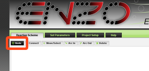
In the Reaction Scheme tab click on Node button (it is already selected by default).
Click inside the white area, to create a node. It will create a green circle like this one:
Now, hold shift on your keyboard, and press E (if the label does not apper, click on node before typing). This will set the label of the node to E:

Nodes with letters represent species.
Create two more nodes, one with a label ES and another one with a label E. You will end up with something like this:

If you want, you can move nodes around by clicking Move/Select button, then click on node and drag around.
Click on Connect button. Click and drag from the left node E to node ES. This will create an arrow between them:
Connect these two nodes in the opposite direction as well:
Now connect node ES with the right node E:
Click on Arc In button and click on k0. Hold shift on your keyboard, and press S. You will end with something like this:
Now, click on Arc Out button and create an S out arc on arrow k1, and a P out arc on arrow k2:

Do not worry if you do something wrong. Just click on Delete button to delete objects, or select an object with the Move/Select button and press backspace on your keyboard to fix mistyped labels.

Step 2: Set Parameters

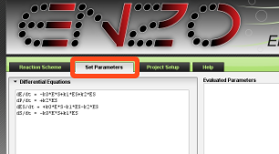
Switch to the Set Parameters tab.
Differential equations are already displayed in the Differential Equations field.

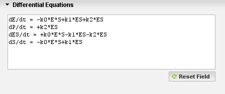
If you change anything on the reaction scheme, you will have to press the Reset Field button to display the changes.
Click on Rate Constants to expand the field.

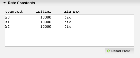
For each rate constant, initial, minimum and maximum rates will be filled with default values: 10000 for initial, fix for min max.

The values do not need to be in any particular units. ENZO will use whatever units are provided.
Change the initial value of k0 to 1.4e6. Leave fix for min max (fixed constants will not be fitted).
Change the initial value of k1 to 14. Set min max to 0 1e20.
Change the initial value of k2 to 9. Set min max to 0 1e20.

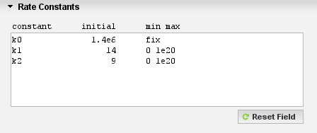
Do not worry about the indentation, it will be automatically corrected when your mouse leaves the field.
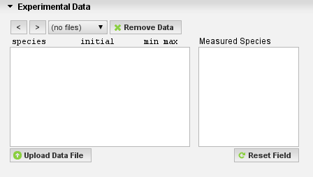
Click on Experimental Data to expand the field.
Click on Upload Data File button, and select the file quickguide.dat.
(Here is the file in case you have not downloaded it: Experimental Data File)

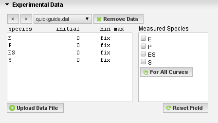
The file will appear in the drop-down menu.

The data of the file will be displayed on the Time Course of the Reaction chart:

Data files are plain text files with two columns separated by space or tab. The first column is the time of the reaction and the second is the concentration of species.

Similar to the rate constants, each species has an initial, minimum and maximum concentration to set.
By default, initial concentrations are 0, and min and max are fixed.
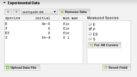
Change the inital concentration of E to 4e-8.
Change the inital concentration of S to 5e-4 and min max to 0 1. Leave the other concentrations as default.
Also, mark P as the measured species.
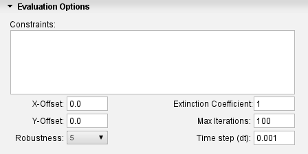
Click on Evaluation Options to expand the field.
Set Max Iterations to 100 and Time Step (dt) to 0.001.

Step 3: Start Evaluation

You may now start the evaluation. Click the big green Start button.

While the evaluation is running, curve fitting is shown in real-time on the Time Course of the Reaction chart.

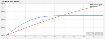
Evaluated parameters are shown approximately every second during the evaluation (depending on the evaluation speed).

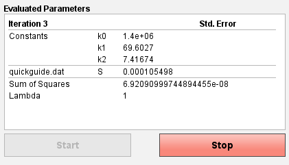
The decreasing lambda value indicates a successful convergence of the fitting procedure.
The sum of squares measures the difference between the measured and the fitted values of the dependent variable.
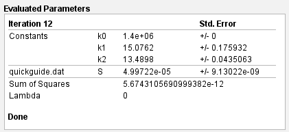
You may stop the evaluation at any time by pressing the Stop button.

When the evaluation finishes, either by converging or by reaching the iteration limit, the final evaluated parameters will be shown.
You can try changing any parameter and see how the evaluation process changes.

This is all for the quick guide! Happy fitting!

Back to Table of Contents