4. Setting Parameters
In order to set the evaluation parameters switch to the Set Parameters tab:
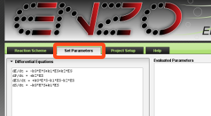
The Set Parameters tab contains sections for the differential equations, rate constants, experimental data and evaluation options. To switch between sections click on the section name.
The Set Parameters tab also displays the evaluated parameters in the Evaluated Parameters field on the right side. This is explained further in Chapter 5 of this help.
Differential Equations
The equations are generated upon drawing the scheme.
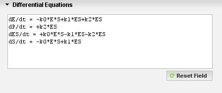
If you modify the scheme after the equations have already been generated, it is necessary to press the Reset Field button. The equations will be regenerated from the new scheme.
If necessary, you can manualy edit the equations. The modified equations will be then be used in the evaluation.
Rate Constants
In the Rate Constants section press the Reset Field button to enter default rate constants values.
For each constant a row is created. In the first column are constants, in the second column are the initial values, and the third column are the minimum and maximum values separated by space.
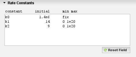
By default for each constant the initial value is 10000, minimum and maximum are 0 and 1e20 respectively.
Minimum and maximum values should be separated by space.
To fix a value, enter the word fix in the min max column. Fixed constants will not be fitted.
The values do not need to be in any particular units. ENZO will use whatever units are provided.
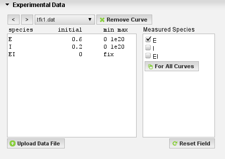
Experimental Data
The Experimental Data section allows you to upload experimental data files from your computer to the server.
File Format of Experimental Data
Experimental data files are plain text files with two columns separated by spaces or tab.
The first column contains time and the second contains the concentration.
Like for rate constants, the values do not need to be in any particular units.
Here is an example of valid content of an experimental data file (first 10 rows are shown):
	2.5           5.44941157025224E-9
	9.75          3.8230586871096E-8
	20            3.24705870766325E-8
	33.1          3.92470574230602E-8
	43            3.9444704474831E-8
	53            4.22258808461774E-8
	70.3          8.22070558901006E-8
	82            9.44470554533355E-8
	93            1.13731760647544E-7
	105           1.35247053997452E-7
Files used in the examples are available as a reference: example1.zip, example2.zip, example3.zip.
Uploading Experimental Data Files
To upload a data file press the Upload Data File button. Use the file browsing window that appears, to select your file.
When the file is uploaded, it appears in the drop down menu and the measured data is shown on the Time Course of the Reaction chart.
If you have multiple data files, you can select multiple files in the file browsing window by holding down the Control key on your keyboard and upload them all at once. This functionality does not work in Internet Explorer, however you may also upload a zip file, containing multiple data files.
For each uploaded file, enter the initial value in the second column and the minimum and the maximum values in the third column. The minimum and maximum values should be separated by space.
To fix a value enter the word fix in the min max column. Fixed species will not be fitted.
You can switch between files by pressing the left (<) and right (>) buttons, or by selecting a file from the drop down menu. To remove a data file press the Remove Data button.
In the Measured Species field, click on the species that are measured (a check appears).
If one measures two or more species at the same time, then one would check more than one box in the measured species. For example, the second column in the upload file can be the sum of concentrations of two species (c(E)+c(I)). In this case one would check E and I.
Evaluation Options
Click on Evaluation Options to expand the section. If necessary change the maximum number of iterations and the time step.
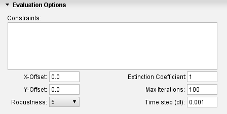
It is also possible to enter evaluation constraints, X and Y data offsets, the extinction coefficient and robustness values
Evaluation Constraints
Evaluation constraints can be used to speed up the evaluation. For complex schemes, constraints may be necessary in order to reach convergence.
Here is an example of valid constraints:
        k13=k3
        k15=k9=k7=k2=k1
        k10=k4*2
The constraints overrule the fixed values. When one has a constraint of e.g. k15=k9=k7=k2=k1 then only the last rate constant (i.e. k1) will be fitted. It is possible to enter multipliers as well.
In the example above:
- k13 will not be fitted and will have the same value as k3.
- k15, k9, k7, and k2 will not be fitted and will have the same value as k1.
- k10 will not be fitted and will have twice the value of k4.
Offset
The X-Offset value defines the time interval between the start of the reaction and the start of the measurement (dead time).
The Y-Offset value defines the putative plateau.
Robustness
The Robustness value determines the allowed changes of fitted parameters at each iteration step.
The fitting of coefficients of differential equations typically starts with higher robustness
values to obtain a rough estimate, which is later refined using lower values to obtain the final local minimum.
Extinction Coefficient
The extinction coefficient converts the absorbance to concentration of a species when there is nothing else in
the sample that absorbs at the wavelength of interest. If, for example, a reactant and product both absorb, then
the relevant value should be specified accordingly.